10주차에는 transformer의 Keras Layers에 대해 배웠다.
강의에서 배운 사고의 흐름을 복습 및 정리하고자 한다.
1. Import
가장 먼저 시작해야 되는 것은, 필요한 라이브러리를 import하는 것이다.
!pip install -q keras-core
import numpy as np numpy
import os
os.environ["KERAS_BACKEND"] = "torch"
import keras_core as keras
import keras_core
keras에 대해 배우는만큼 keras나 numpy를 import하는 것은 딱히 의외인 것은 아니다.
os.environ["KERAS_BACKEND"] = "torch"를 입력하여 KERAS_BACKEND을 torch로 설정하였다.
케라스(Keras)는 다양한 백엔드 엔진을 지원하는데, 이 설정은 PyTorch를 백엔드로 사용하도록 지정한 것이다.
2. Embedding Layer
Embedding Layer는 말 그대로 embedding 역할을 수행하는 layer를 말한다.
자연어로 입력된 input이 encoding 되면, 이를 vector로 embedding 하여 다음 layer로 넘겨주는 역할이다.
따라서, embedding vector 및 embedding layer 모두 학습 대상이다.
그림으로 살펴보면 다음과 같다
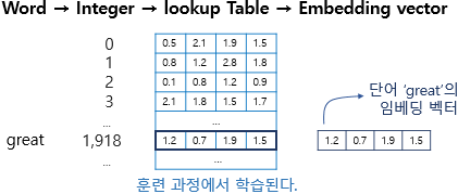
embedding layer의 원리
이제 code로 살펴보도록 하겠다.
model = keras_core.Sequential()
9주차에서와는 달리, keras_core.Sequential 함수를 이용해 새로운 model을 생성하였다.
layer를 선형 스택으로 쌓는 방식이다.
model.add(keras_core.layers.Embedding(1000, 64))
위에서 만든 model에 embedding layer를 추가해주었다.
여기서 1000은 입력 가능한 최대 크기(단어의 수)이고, 64는 embedding vector의 차원 크기를 말한다.
input_array = np.random.randint(1000, size=(32, 10))
model.compile('rmsprop', 'mse')
output_array = model.predict(input_array)
numpy의 random.randint로 생성된 0~999까지의 정수로 이루어진 32x10 행렬을 input array로 설정하였다.
이후 optimizer인 rmsprop와 손실함수인 mse를 설정하여 model은 compile 한 후,
compile된 모델에 input array를 입력으로 설정해 두었다.
출력은 output_array로 하여, 모델의 기초적인 틀을 갖추어 두었다.
emb = keras.layers.Embedding(100,2)
x = np.random.randint(0,100, (2,10))
다시 embedding layer로 돌아와, embedding layer에 대해서 보다 쉽게 이해하도록 emb라는 layer를 만들었다.
앞에와 동일하게, 100은 입력 가능한 최대 단어의 수를 의미하고, 2는 embedding vector의 차원 크기를 말한다.
x는 input으로 들어갈 행렬으로, 0~99까지의 정수로 random하게 생성된 2x10 행렬이다.
emb(x)
실제로 emb에 x를 넣어보면, 아래와 같은 결과가 나오는 것을 볼 수 있다.
random한 정수를 embedding한 것이다.

emb = keras.layers.Embedding(vocab_size, d_model)
뒤에서 emb를 다시 사용할 것이므로, 수치를 초기화해 두었다.
지금까지의 과정: "input 행렬 -> embedding layer"
3. Dense Layer
Dense Layer는 이전 Layer(Embedding Layer)로부터 Input을 받아, 다음 Layer로 Output을 보내주는 역할을 수행한다.
그 원리를 그림으로 살펴보면 다음과 같다.

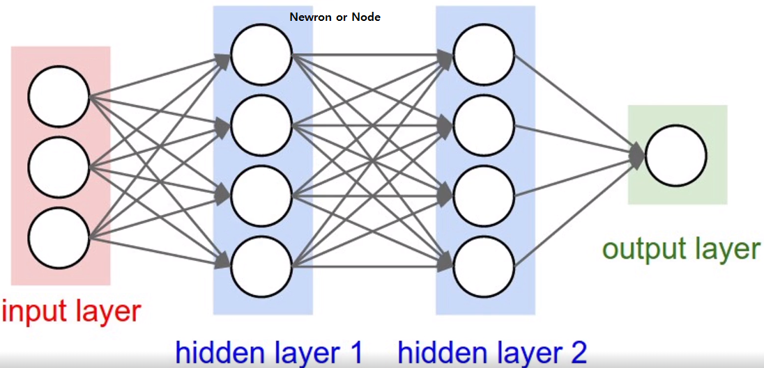
Dense Layer는 Hidden Layer를 만드는 데에 사용되지만, 모든 Hidden Layer가 Dense Layer로 만들어진 것은 아니다.
이제 Code로 살펴보도록 하겠다.
keras.layers.Dense(5)
linear = keras.layers.Dense(5)
Dense Layer를 생성해 linear라는 변수에 할당했다.
다만 model에 추가한 것은 아니고, 그냥 만들어 linear에 넣기만 한 것이다.
여기서 5는 Layer의 출력 차원의 크기를 의미한다.
linear 2= keras.layers.Dense(5)
이런식으로 linear 2, linear3를 만들면, layer를 계속 늘릴 수 있다.
Embedding Layer -> Dense Layer이니만큼,
이제 input에 Embedding Layer가 들어가도록 해야 한다.
emb = keras.layers.Embedding(100, 512)
x = np.random.randint(0, 100, (2000, 10))
앞에서 만들어둔 emb와 x를 다시 사용하였다.
이번엔 최대 입력 가능 단어를 100개로, embedding vector의 차원을 512로 두었다.
x는 0~99까지의 random한 정수로 이루어진 2000x10의 행렬이다.
x_emb = emb(x)
x_emb.shape
emb layer에 x를 input으로 넣었다.
x_emb의 차원은 2000 x 10 x 512이다.
linear3 = keras.layers.Dense(5)
linear3(x_emb)
이렇게 한다면, embedding layer가 dense layer로 들어가는 방식을 구성할 수 있다.
지금까지의 과정: "input 행렬 -> embedding layer -> dense layer"
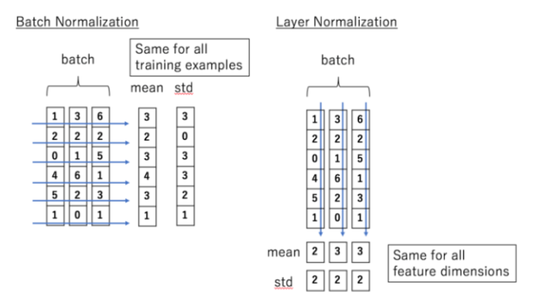
4. Layer Normalization
Layer Normalization은 input의 평균과 분산을 사용해 layer의 입력을 정규화한다.
그 원리를 그림으로 살펴보면 다음과 같다.
이제 Code로 살펴보도록 하겠다.
layernorm = keras.layers.LayerNormalization()
LayerNormalizatinon Layer를 생성해 layernorm이라는 변수에 할당했다.
다만 모델이 추가한 것은 아니고, 그냥 만들어 layernorm에 넣기만 한 것이다.
emb = keras.layers.Embedding(100, 512)
linear = keras.layers.Dense(5)
x = np.random.randint(0, 100, (2, 10))
x_emb = emb(x)
x_lin = linear(x_emb)
앞에서 수행한 과정을 반복하였다.
embedding layer와 dense layer를 만들었고,
2x10의 행렬이 -> embedding layer를 거쳐 -> dense layer로 들어가도록 하였다.
layernorm(x_lin)
x_lin은 dense layer까지 통과한 상태이다.
이 x_lin을 layernorm에 넣어주면, x_lin을 정규화시킬 수 있다.
정규화 결과는 다음과 같다.

이렇게 한다면, embedding layer가 dense layer를 거친 후 정규화되는 방식을 구성할 수 있다.
지금까지의 과정: "input 행렬 -> embedding layer -> dense layer -> layer normalization"
6. Add Layer
Add layer는 두 개 이상의 input을 받아 그것들을 element-wise하게 더하는 데 사용된다.
Code로 살펴보도록 하겠다.
add = keras.layers.Add()
add layer를 생성해 add라는 변수에 할당했다.
여기서도 마찬가지로, 모델이 추가한 것은 아니고 그냥 만들어 add에 넣기만 한 것이다.
x_emb = emb(x)
x_lin = linear(x_emb)
x_norm = layernorm(x_lin)
앞에서 수행한 과정을 반복하였다.
2x10의 행렬이 -> embedding layer를 거쳐 -> dense layer를 거친 후 -> layer normalization이 되도록 하였다.
layer normalization이 된 것을 x_norm에 저장하였다.
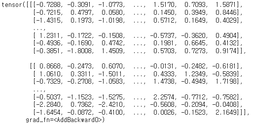
add([x_lin, x_norm])
add layer에 x_norm과 x_lin을 넣어주었다.
add layer는 두 요소의 합을 element wise로 계산한다.
결과를 출력해보면 다음과 같다.

이렇게 한다면, dense layer와 dense layer가 정규화된 layer가 add layer를 통과하는 방식을 구성할 수 있다.
지금까지의 과정: "input 행렬 -> embedding layer -> dense layer -> layer normalization -> add layer"
7. Dropout Layer
Dropout layer는 hidden layer의 노드 일부를 drop 하는 layer이다.
노드를 떨어지면 model의 성능이 떨어지지 않을까 우려할 수 있지만,
dropout이 적절하게 이루어지면 overfitting이 방지되므로 오히려 성능 향상에 도움이 된다.
그 원리를 그림으로 살펴보면 다음과 같다

이제는 Code로 살펴보도록 하겠다.
dropout = keras.layers.Dropout(0.2)
dropout layer를 생성해 dropout 변수에 할당했다.
여기서도 마찬가지로, 모델이 추가한 것은 아니고 그냥 만들어 dropout에 넣기만 한 것이다.
또한 0.2는 dropout 비율을 말한다. 전체 노드의 0.2%를 버리겠다는 뜻이다.
dropout(x_lin, training=True)
앞에서 사용하였던 dense layer에 dropout를 적용하였다.
여기서 training=True는, 이 dropout이 train 중에만 적용되며 test 중에는 일어나지 않음을 말한다.
결과를 출력해보면 다음과 같다.

이렇게 한다면, dense layer에 dropout layer를 적용하여 overfitting을 방지하도록 할 수 있다.
지금까지의 과정: "input 행렬 -> embedding layer -> dense layer -> layer normalization -> add layer -> dropout layer"
8. Feed Forward Network
Feed Forward Network는 input부터 output까지 한 방향으로만 정보가 전달되는 network이다.
아래 그림을 보면, 그 원리를 보다 쉽게 파악할 수 있다.
왼쪽에서 오른쪽으로, 한 방향으로만 정보가 전달되는 것을 확인할 수 있다.
지금까지 배웠던 layer들을 총 규합하여 Feed Forward Network를 구성할 것이다.
code로 살펴보도록 하겠다.
linear1 = keras.layers.Dense(2024, activation="relu")
linear2 = keras.layers.Dense(512)
dropout = keras.layers.Dropout(0.1)
add = keras.layers.Add()
layernorm = keras.layers.LayerNormalization()
x = np.random.randn(2,10,512)
이 부분은 위에서 배운 것의 반복이다.
x_seq = dropout(linear2(linear1(x)))
x를 input으로 하여 linear1에 적용한 후, 그 output을 linear2의 input으로 사용했다.
linear2의 output에 dropout layer를 적용한 후, 그 output을 x_seq에 저장하였다.
layernorm(add([x, x_seq]))
기존의 input x와 위에서 구한 x_seq을 input으로 사용하여 add를 적용한 후,
output에 layernorm을 적용한 것이다.
출력해보면 아래와 같다.
같은 논리를 보다 멋지게 정리하면 아래와 같다.
class ffn(keras.layers.Layer):
def __init__(self):
super().__init__()
self.linear1 = keras.layers.Dense(2024, activation="relu")
self.linear2 = keras.layers.Dense(512)
self.dropout = keras.layers.Dropout(0.1)
self.add = keras.layers.Add()
self.layernorm = keras.layers.LayerNormalization()
def call(self, inputs):
x = self.linear1(inputs)
x = self.linear2(x)
x = self.dropout(x)
x = self.add([inputs, x])
return self.layernorm(x)
ffn이라는 feed-forward neural network class를 정의하였다.
이 class에서는 2개의 dense layer, dropout layer, add layer, layernormalization layer가 들어가 있다.
call method는 이러한 layer들을 사용해 input data를 변환해 나간다.
my_ff = ffn()
ffn을 사용하여 최종적으로 my_fff를 만들었다.
x를 정의한 후, my_ff(x)를 실행시키면 나만의 feed forward network를 얻을 수 있다.
x = np.random.randn(4,24,512)
x를 이렇게 정의해 보았다.
my_ff(x)를 실행시켜보면

위와 같이 정상적으로 출력되는 것을 볼 수 있다.
마지막으로 my_ff(x).shape를 출력해봐도,

차원의 크기가 설정해둔대로 잘 되어있는 것을 볼 수 있다.
'Coding' 카테고리의 다른 글
| 경제학코딩2 14주차 - Decoder (2) | 2024.01.21 |
|---|---|
| 경제학코딩2 13주차 - Scaled_dot_product_attention (0) | 2024.01.21 |
| 경제학코딩2 12주차 - Encoder (0) | 2024.01.20 |
| 경제학코딩2 11주차 - Tokenizer & Data Section (0) | 2024.01.20 |
| 경제학코딩2 9주차 - What is torch.nn really? (0) | 2024.01.19 |